 |
|---|
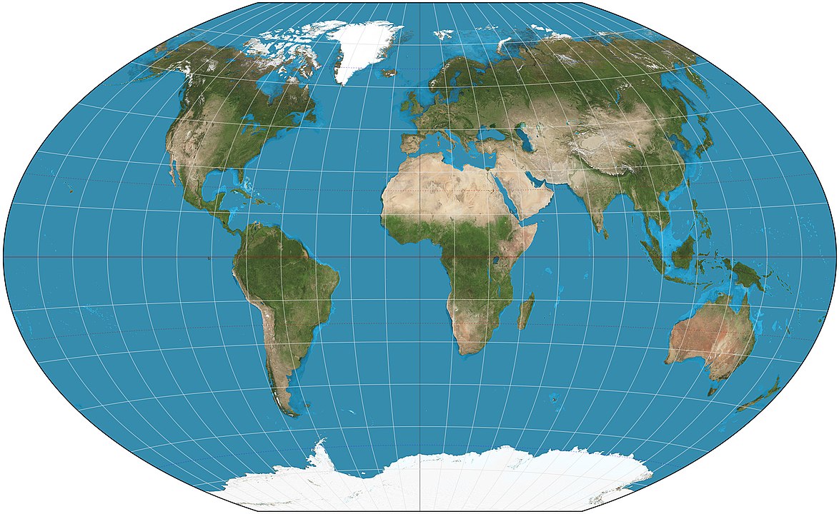
| Winkel tripel projection. Image obtained here |
In this notebook, we use sqlite to investigate tables in the database factbook.db. This data comes from the CIA World Factbook.
As we'll see in the cells below, this database contains demographic information about various countries. Our primary goal for this notebook is to investigate how a country's death rate (number of deaths per 1000 people) relates to other demographic characteristics of the country, such as population density, and birth rate.
We begin by investigating the tables in the databse, and peforming some "reality checks" to make sure nothing is seriously wrong with the data. We then use SQL queries to generate some interesting features. Namely, we compute population density, as well as expected increase in population. Finally, using these features, we take a closer look at how death rate is connected to the other information.
Without further ado, let's begin!
|
|---|
| Winkel tripel projection. Image obtained here |
We begin by loading sqlite, so that our SQL queries will work in this notebook, as well as the database, "factbook.db."
%%capture
%load_ext sql
%sql sqlite:///data/factbook.db
Now we're ready to take a look at the tables in the database.
%%sql
SELECT *
  FROM sqlite_master
 WHERE type='table';
 * sqlite:///data/factbook.db
Done.
| type | name | tbl_name | rootpage | sql |
|---|---|---|---|---|
| table | sqlite_sequence | sqlite_sequence | 3 | CREATE TABLE sqlite_sequence(name,seq) |
| table | facts | facts | 47 | CREATE TABLE "facts" ("id" INTEGER PRIMARY KEY AUTOINCREMENT NOT NULL, "code" varchar(255) NOT NULL, "name" varchar(255) NOT NULL, "area" integer, "area_land" integer, "area_water" integer, "population" integer, "population_growth" float, "birth_rate" float, "death_rate" float, "migration_rate" float) |
In this notebook, we are concerned "facts" table. The other table is created when using sqlite to access the database, so we don't need to worry about it. Let's investigate the first few rows of the facts table.
%%sql
SELECT *
  FROM facts
 LIMIT 5;
 * sqlite:///data/factbook.db
Done.
| id | code | name | area | area_land | area_water | population | population_growth | birth_rate | death_rate | migration_rate |
|---|---|---|---|---|---|---|---|---|---|---|
| 1 | af | Afghanistan | 652230 | 652230 | 0 | 32564342 | 2.32 | 38.57 | 13.89 | 1.51 |
| 2 | al | Albania | 28748 | 27398 | 1350 | 3029278 | 0.3 | 12.92 | 6.58 | 3.3 |
| 3 | ag | Algeria | 2381741 | 2381741 | 0 | 39542166 | 1.84 | 23.67 | 4.31 | 0.92 |
| 4 | an | Andorra | 468 | 468 | 0 | 85580 | 0.12 | 8.13 | 6.96 | 0.0 |
| 5 | ao | Angola | 1246700 | 1246700 | 0 | 19625353 | 2.78 | 38.78 | 11.49 | 0.46 |
We can see this table contains geographic and demographic information by country. For convenenience, here is a table containing descriptions of each column.
| Column Name | Description |
|---|---|
| code | abbreviation for the country name |
| name | name of the country |
| area | country's total area (square kilometers) |
| area_land | country's land area (square kilometers) |
| area_water | country's water area (square kilometers) |
| population | country's population |
| population_growth | country's population growth (percentage) |
| birth_rate | number of births per year per 1,000 people |
| death_rate | number of deaths per year per 1,000 people |
| migration_rate | number of migrants per 1,000 people |
In this section, we begin by writing some queries which serve as basic "reality checks" regarding the data. The first reality check we perform has to do with total area. We want to make sure that the land area and water area add up to the total area. We can answer this with a query.
%%sql
SELECT name, area, area_land, area_water, area - area_land - area_water AS area_difference
   FROM facts
  WHERE area_difference != 0;
 * sqlite:///data/factbook.db
Done.
| name | area | area_land | area_water | area_difference |
|---|---|---|---|---|
| Saint Helena, Ascension, and Tristan da Cunha | 308 | 122 | 0 | 186 |
Saint Helena, Ascension, and Tristan da Cunha is a British overseas territory consisting of the island chain Tristan da Cunha, as well as two separate islands (Saint Helena and Ascension Island). To learn more about this territory, take a look here or here.
After doing some digging, it appears that the above discrepency is due to some data being collected separately for each of Saint Helena, Ascension, and Tristan da Cunha. For instance, it appears that the land area of Saint Helena alone is given by 122 km$^2$. Since the exact land area / water area is unclear from an initial google search, we'll just make note of this discrepency, as the purpose of this notebook is simply to investigate the dataset using queries. If further analyzation was to be done, then this row is a candidate for dropping after reading the query into a pandas dataframe.
 |
|---|
| Atlas of Saint Helena, Ascension, and Tristan da Cunha. Image obtained here |
The next thing we'll investigate is maximum and minimum of a few columns. Some things to look for are the following: each rate out of 1,000 people should be less than 1,000, and greater than 0. We'll also be looking for a maximum population which seems reasonable.
%%sql
SELECT MAX(population), MIN(population), MAX(birth_rate), MIN(birth_rate), MAX(death_rate), MIN(death_rate), MAX(migration_rate), MIN(migration_rate)
   FROM facts;
 * sqlite:///data/factbook.db
Done.
| MAX(population) | MIN(population) | MAX(birth_rate) | MIN(birth_rate) | MAX(death_rate) | MIN(death_rate) | MAX(migration_rate) | MIN(migration_rate) |
|---|---|---|---|---|---|---|---|
| 7256490011 | 0 | 45.45 | 6.65 | 14.89 | 1.53 | 22.39 | 0.0 |
We first note that since the minimum of migration_rate is 0, this value does not denote net migration rate. This impacts our analysis in a later section, when we estimate the change in population. The only other suspcious things are the minimum population of 0, and maximum population of 7 Billion. Let's take a closer look at these.
%%sql
SELECT name, MAX(population)
   FROM facts;
 * sqlite:///data/factbook.db
Done.
| name | MAX(population) |
|---|---|
| World | 7256490011 |
We can see from this that the world is included as an entry. Let's take a look at the most populous country by excluding the row corresponding to the world.
%%sql
SELECT name, MAX(population)
   FROM facts
  WHERE name != 'World';
 * sqlite:///factbook.db
Done.
| name | MAX(population) |
|---|---|
| China | 1367485388 |
The above result is much more reasonable. Now that we've made sense of a maximum population of 7 Billion, let's look at which Country has a minimum population of 0.
%%sql
SELECT name, population
   FROM facts
  WHERE population = 0;
 * sqlite:///data/factbook.db
Done.
| name | population |
|---|---|
| Antarctica | 0 |
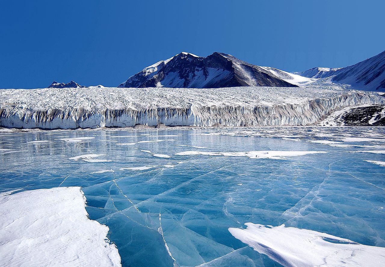
According to the CIA Factbook Antarctica page, we see that there are no natives to Antarctica, and the population is indeed 0. At any given time, however, there are likely a few thousand temporary researchers living in Antarctica.
 |
|---|
| Blue ice covering Lake Fryxell, in the Transantarctic Mountains. Image obtained here |
In this section, we investigate population density. In particular, we first write a query that computes population density as a column. Then, we study countries with high population density, as well as low population density. $$ \textrm{population density } = \frac{\textrm{population}}{\textrm{area}} $$.
%%sql
SELECT *, ROUND(CAST(population AS float)/CAST(area AS float),2) AS population_density
   FROM facts
  ORDER BY population_density DESC
 LIMIT 10;
 * sqlite:///data/factbook.db
Done.
| id | code | name | area | area_land | area_water | population | population_growth | birth_rate | death_rate | migration_rate | population_density |
|---|---|---|---|---|---|---|---|---|---|---|---|
| 205 | mc | Macau | 28 | 28 | 0 | 592731 | 0.8 | 8.88 | 4.22 | 3.37 | 21168.96 |
| 117 | mn | Monaco | 2 | 2 | 0 | 30535 | 0.12 | 6.65 | 9.24 | 3.83 | 15267.5 |
| 156 | sn | Singapore | 697 | 687 | 10 | 5674472 | 1.89 | 8.27 | 3.43 | 14.05 | 8141.28 |
| 204 | hk | Hong Kong | 1108 | 1073 | 35 | 7141106 | 0.38 | 9.23 | 7.07 | 1.68 | 6445.04 |
| 251 | gz | Gaza Strip | 360 | 360 | 0 | 1869055 | 2.81 | 31.11 | 3.04 | 0.0 | 5191.82 |
| 233 | gi | Gibraltar | 6 | 6 | 0 | 29258 | 0.24 | 14.08 | 8.37 | 3.28 | 4876.33 |
| 13 | ba | Bahrain | 760 | 760 | 0 | 1346613 | 2.41 | 13.66 | 2.69 | 13.09 | 1771.86 |
| 108 | mv | Maldives | 298 | 298 | 0 | 393253 | 0.08 | 15.75 | 3.89 | 12.68 | 1319.64 |
| 110 | mt | Malta | 316 | 316 | 0 | 413965 | 0.31 | 10.18 | 9.09 | 1.98 | 1310.02 |
| 227 | bd | Bermuda | 54 | 54 | 0 | 70196 | 0.5 | 11.33 | 8.23 | 1.88 | 1299.93 |
We first notice that some of the most densely populated areas correspond to countries with incredibly small area. Let's instead take a look at the 10 most densely populated countries with above average area.
%%sql
SELECT *, ROUND(CAST(population AS float)/CAST(area AS float),2) AS population_density
   FROM facts
  WHERE area > (SELECT AVG(area)
                   FROM facts)
ORDER BY population_density DESC
LIMIT 10;
 * sqlite:///data/factbook.db
Done.
| id | code | name | area | area_land | area_water | population | population_growth | birth_rate | death_rate | migration_rate | population_density |
|---|---|---|---|---|---|---|---|---|---|---|---|
| 77 | in | India | 3287263 | 2973193 | 314070 | 1251695584 | 1.22 | 19.55 | 7.32 | 0.04 | 380.77 |
| 132 | pk | Pakistan | 796095 | 770875 | 25220 | 199085847 | 1.46 | 22.58 | 6.49 | 1.54 | 250.08 |
| 129 | ni | Nigeria | 923768 | 910768 | 13000 | 181562056 | 2.45 | 37.64 | 12.9 | 0.22 | 196.55 |
| 37 | ch | China | 9596960 | 9326410 | 270550 | 1367485388 | 0.45 | 12.49 | 7.53 | 0.44 | 142.49 |
| 78 | id | Indonesia | 1904569 | 1811569 | 93000 | 255993674 | 0.92 | 16.72 | 6.37 | 1.16 | 134.41 |
| 197 | ee | European Union | 4324782 | None | None | 513949445 | 0.25 | 10.2 | 10.2 | 2.5 | 118.84 |
| 61 | fr | France | 643801 | 640427 | 3374 | 66553766 | 0.43 | 12.38 | 9.16 | 1.09 | 103.38 |
| 179 | tu | Turkey | 783562 | 769632 | 13930 | 79414269 | 1.26 | 16.33 | 5.88 | 2.16 | 101.35 |
| 58 | et | Ethiopia | 1104300 | None | 104300 | 99465819 | 2.89 | 37.27 | 8.19 | 0.22 | 90.07 |
| 53 | eg | Egypt | 1001450 | 995450 | 6000 | 88487396 | 1.79 | 22.9 | 4.77 | 0.19 | 88.36 |
Many results above correspond to countries which are very well known to be densely populated, such as India and China.
Now, let's take a look at countries with a low population density.
%%sql
SELECT *, ROUND(CAST(population AS float)/CAST(area AS float),2) AS population_density
   FROM facts
  WHERE area > (SELECT AVG(area)
                   FROM facts )
 ORDER BY population_density ASC
LIMIT 10;
 * sqlite:///data/factbook.db
Done.
| id | code | name | area | area_land | area_water | population | population_growth | birth_rate | death_rate | migration_rate | population_density |
|---|---|---|---|---|---|---|---|---|---|---|---|
| 207 | gl | Greenland | 2166086 | 2166086 | None | 57733 | 0.0 | 14.48 | 8.49 | 5.98 | 0.03 |
| 118 | mg | Mongolia | 1564116 | 1553556 | 10560 | 2992908 | 1.31 | 20.25 | 6.35 | 0.84 | 1.91 |
| 122 | wa | Namibia | 824292 | 823290 | 1002 | 2212307 | 0.59 | 19.8 | 13.91 | 0.0 | 2.68 |
| 9 | as | Australia | 7741220 | 7682300 | 58920 | 22751014 | 1.07 | 12.15 | 7.14 | 5.65 | 2.94 |
| 112 | mr | Mauritania | 1030700 | 1030700 | 0 | 3596702 | 2.23 | 31.34 | 8.2 | 0.83 | 3.49 |
| 32 | ca | Canada | 9984670 | 9093507 | 891163 | 35099836 | 0.75 | 10.28 | 8.42 | 5.66 | 3.52 |
| 100 | ly | Libya | 1759540 | 1759540 | 0 | 6411776 | 2.23 | 18.03 | 3.58 | 7.8 | 3.64 |
| 23 | bc | Botswana | 581730 | 566730 | 15000 | 2182719 | 1.21 | 20.96 | 13.39 | 4.56 | 3.75 |
| 87 | kz | Kazakhstan | 2724900 | 2699700 | 25200 | 18157122 | 1.14 | 19.15 | 8.21 | 0.41 | 6.66 |
| 143 | rs | Russia | 17098242 | 16377742 | 720500 | 142423773 | 0.04 | 11.6 | 13.69 | 1.69 | 8.33 |
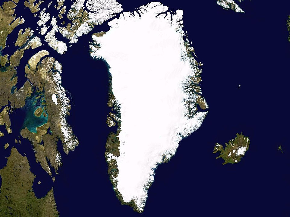
We again recognize these results as making sense. Note that Greenland's population density is nearly 200 times smaller than Mongolia, the country with the next smallest population density. That is quite the outlier!
 |
|---|
| Greenland from space. Image obtained here. |
In this section, we'll write a query showing which countries have the highest and lowest expected increase in population.
The following equation estimates the increase in population for a given country:
$$ \textrm{ increase in population } = \left(\textrm{birth rate}\right) \times \left( \textrm{people} \right) - \left( \textrm{death rate} \right) \times \left(\textrm{people}\right) $$$$ + \left(\textrm{net migration rate} \right) \times \left( \textrm{people} \right). $$Unfortuntately, this database does not contain the net migration rate. The migration rate reported seems to be the absolute value of net migration rate. Since in general we cannot tell which countries have more immigrants than emigrants (and vice versa), we will just ignore the last term, and base our calculation purely on birth and death rates.
Note that since the birth and death rates reported are per 1,000 people, we have to convert each population to thousands of people. Here is our query calculating this.
%%sql
SELECT *, ROUND((birth_rate - death_rate)*(CAST(population AS float)/CAST(1000 AS float)),2) AS population_increase
   FROM facts
  WHERE name != 'World'
 ORDER BY population_increase DESC
LIMIT 10;
 * sqlite:///data/factbook.db
Done.
| id | code | name | area | area_land | area_water | population | population_growth | birth_rate | death_rate | migration_rate | population_increase |
|---|---|---|---|---|---|---|---|---|---|---|---|
| 77 | in | India | 3287263 | 2973193 | 314070 | 1251695584 | 1.22 | 19.55 | 7.32 | 0.04 | 15308236.99 |
| 37 | ch | China | 9596960 | 9326410 | 270550 | 1367485388 | 0.45 | 12.49 | 7.53 | 0.44 | 6782727.52 |
| 129 | ni | Nigeria | 923768 | 910768 | 13000 | 181562056 | 2.45 | 37.64 | 12.9 | 0.22 | 4491845.27 |
| 132 | pk | Pakistan | 796095 | 770875 | 25220 | 199085847 | 1.46 | 22.58 | 6.49 | 1.54 | 3203291.28 |
| 58 | et | Ethiopia | 1104300 | None | 104300 | 99465819 | 2.89 | 37.27 | 8.19 | 0.22 | 2892466.02 |
| 78 | id | Indonesia | 1904569 | 1811569 | 93000 | 255993674 | 0.92 | 16.72 | 6.37 | 1.16 | 2649534.53 |
| 14 | bg | Bangladesh | 148460 | 130170 | 18290 | 168957745 | 1.6 | 21.14 | 5.61 | 0.46 | 2623913.78 |
| 40 | cg | Congo, Democratic Republic of the | 2344858 | 2267048 | 77810 | 79375136 | 2.45 | 34.88 | 10.07 | 0.27 | 1969297.12 |
| 138 | rp | Philippines | 300000 | 298170 | 1830 | 100998376 | 1.61 | 24.27 | 6.11 | 2.09 | 1834130.51 |
| 114 | mx | Mexico | 1964375 | 1943945 | 20430 | 121736809 | 1.18 | 18.78 | 5.26 | 1.68 | 1645881.66 |
This estimate makes sense, though including the net migration would make it more accurate. India and China are well known to be among the fastest growing countries. Now lets look at the countries growing the least.
%%sql
SELECT *, ROUND((birth_rate - death_rate)*(CAST(population AS float)/CAST(1000 AS float)),2) AS population_increase
   FROM facts
  WHERE name != 'World' AND population_increase != 'None'
 ORDER BY population_increase ASC
LIMIT 10;
 * sqlite:///data/factbook.db
Done.
| id | code | name | area | area_land | area_water | population | population_growth | birth_rate | death_rate | migration_rate | population_increase |
|---|---|---|---|---|---|---|---|---|---|---|---|
| 143 | rs | Russia | 17098242 | 16377742 | 720500 | 142423773 | 0.04 | 11.6 | 13.69 | 1.69 | -297665.69 |
| 65 | gm | Germany | 357022 | 348672 | 8350 | 80854408 | 0.17 | 8.47 | 11.42 | 1.24 | -238520.5 |
| 85 | ja | Japan | 377915 | 364485 | 13430 | 126919659 | 0.16 | 7.93 | 9.51 | 0.0 | -200533.06 |
| 183 | up | Ukraine | 603550 | 579330 | 24220 | 44429471 | 0.6 | 10.72 | 14.46 | 2.25 | -166166.22 |
| 83 | it | Italy | 301340 | 294140 | 7200 | 61855120 | 0.27 | 8.74 | 10.19 | 4.1 | -89689.92 |
| 142 | ro | Romania | 238391 | 229891 | 8500 | 21666350 | 0.3 | 9.14 | 11.9 | 0.24 | -59799.13 |
| 26 | bu | Bulgaria | 110879 | 108489 | 2390 | 7186893 | 0.58 | 8.92 | 14.44 | 0.29 | -39671.65 |
| 75 | hu | Hungary | 93028 | 89608 | 3420 | 9897541 | 0.22 | 9.16 | 12.73 | 1.33 | -35334.22 |
| 153 | ri | Serbia | 77474 | 77474 | 0 | 7176794 | 0.46 | 9.08 | 13.66 | 0.0 | -32869.72 |
| 67 | gr | Greece | 131957 | 130647 | 1310 | 10775643 | 0.01 | 8.66 | 11.09 | 2.32 | -26184.81 |
While these values are quite interesting, it may be more informative to study this quantity as a percentage of the total population. Let's take a look.
%%sql
SELECT *, ROUND((birth_rate - death_rate)*(CAST(population AS float)/CAST(1000 AS float)),2) AS population_increase,
       ROUND(birth_rate - death_rate,2) AS population_increase_rate
   FROM facts
  WHERE name != 'World' AND population_increase != 'None'
 ORDER BY population_increase_rate ASC
LIMIT 10;
 * sqlite:///data/factbook.db
Done.
| id | code | name | area | area_land | area_water | population | population_growth | birth_rate | death_rate | migration_rate | population_increase | population_increase_rate |
|---|---|---|---|---|---|---|---|---|---|---|---|---|
| 26 | bu | Bulgaria | 110879 | 108489 | 2390 | 7186893 | 0.58 | 8.92 | 14.44 | 0.29 | -39671.65 | -5.52 |
| 153 | ri | Serbia | 77474 | 77474 | 0 | 7176794 | 0.46 | 9.08 | 13.66 | 0.0 | -32869.72 | -4.58 |
| 96 | lg | Latvia | 64589 | 62249 | 2340 | 1986705 | 1.06 | 10.0 | 14.31 | 6.26 | -8562.7 | -4.31 |
| 102 | lh | Lithuania | 65300 | 62680 | 2620 | 2884433 | 1.04 | 10.1 | 14.27 | 6.27 | -12028.09 | -4.17 |
| 183 | up | Ukraine | 603550 | 579330 | 24220 | 44429471 | 0.6 | 10.72 | 14.46 | 2.25 | -166166.22 | -3.74 |
| 75 | hu | Hungary | 93028 | 89608 | 3420 | 9897541 | 0.22 | 9.16 | 12.73 | 1.33 | -35334.22 | -3.57 |
| 65 | gm | Germany | 357022 | 348672 | 8350 | 80854408 | 0.17 | 8.47 | 11.42 | 1.24 | -238520.5 | -2.95 |
| 158 | si | Slovenia | 20273 | 20151 | 122 | 1983412 | 0.26 | 8.42 | 11.37 | 0.37 | -5851.07 | -2.95 |
| 142 | ro | Romania | 238391 | 229891 | 8500 | 21666350 | 0.3 | 9.14 | 11.9 | 0.24 | -59799.13 | -2.76 |
| 44 | hr | Croatia | 56594 | 55974 | 620 | 4464844 | 0.13 | 9.45 | 12.18 | 1.39 | -12189.02 | -2.73 |
We remark the this ordering is likely to change significantly if we were able to factor in migration. For instance, Latvia and Lithuania both have migration_rate $\approx 6$. After factoring this in, it would shift their standing to the smallest population_increase_rate, considering both these countries have a negative net migration (as seen on the CIA factbook website).
Let's begin to take a closer look at death rate by using this to order the countries.
%%sql
SELECT *, ROUND(CAST(population AS float)/CAST(area AS float),2) AS population_density
   FROM facts
  WHERE area > (SELECT AVG(area)
                   FROM facts ) AND name != 'World'
 ORDER BY death_rate DESC
LIMIT 10;
 * sqlite:///factbook.db
Done.
| id | code | name | area | area_land | area_water | population | population_growth | birth_rate | death_rate | migration_rate | population_density |
|---|---|---|---|---|---|---|---|---|---|---|---|
| 183 | up | Ukraine | 603550 | 579330 | 24220 | 44429471 | 0.6 | 10.72 | 14.46 | 2.25 | 73.61 |
| 122 | wa | Namibia | 824292 | 823290 | 1002 | 2212307 | 0.59 | 19.8 | 13.91 | 0.0 | 2.68 |
| 1 | af | Afghanistan | 652230 | 652230 | 0 | 32564342 | 2.32 | 38.57 | 13.89 | 1.51 | 49.93 |
| 34 | ct | Central African Republic | 622984 | 622984 | 0 | 5391539 | 2.13 | 35.08 | 13.8 | 0.0 | 8.65 |
| 143 | rs | Russia | 17098242 | 16377742 | 720500 | 142423773 | 0.04 | 11.6 | 13.69 | 1.69 | 8.33 |
| 160 | so | Somalia | 637657 | 627337 | 10320 | 10616380 | 1.83 | 40.45 | 13.62 | 8.49 | 16.65 |
| 23 | bc | Botswana | 581730 | 566730 | 15000 | 2182719 | 1.21 | 20.96 | 13.39 | 4.56 | 3.75 |
| 129 | ni | Nigeria | 923768 | 910768 | 13000 | 181562056 | 2.45 | 37.64 | 12.9 | 0.22 | 196.55 |
| 109 | ml | Mali | 1240192 | 1220190 | 20002 | 16955536 | 2.98 | 44.99 | 12.89 | 2.26 | 13.67 |
| 194 | za | Zambia | 752618 | 743398 | 9220 | 15066266 | 2.88 | 42.13 | 12.67 | 0.68 | 20.02 |
We immediately see that many countries with high values of death_rate currently have serious conflicts going on either within or near their boarders. Interestingly, we also notice that, with the exception of Ukraine,Namibia, and Russia, the countries with the highest death rates also have high birth rates. Lets investigate this further by ordering by birth_rate.
%%sql
SELECT *, ROUND(CAST(population AS float)/CAST(area AS float),2) AS population_density
   FROM facts
  WHERE area > (SELECT AVG(area)
                   FROM facts ) AND name != 'World'
 ORDER BY birth_rate DESC
LIMIT 10;
 * sqlite:///factbook.db
Done.
| id | code | name | area | area_land | area_water | population | population_growth | birth_rate | death_rate | migration_rate | population_density |
|---|---|---|---|---|---|---|---|---|---|---|---|
| 109 | ml | Mali | 1240192 | 1220190 | 20002 | 16955536 | 2.98 | 44.99 | 12.89 | 2.26 | 13.67 |
| 194 | za | Zambia | 752618 | 743398 | 9220 | 15066266 | 2.88 | 42.13 | 12.67 | 0.68 | 20.02 |
| 160 | so | Somalia | 637657 | 627337 | 10320 | 10616380 | 1.83 | 40.45 | 13.62 | 8.49 | 16.65 |
| 5 | ao | Angola | 1246700 | 1246700 | 0 | 19625353 | 2.78 | 38.78 | 11.49 | 0.46 | 15.74 |
| 121 | mz | Mozambique | 799380 | 786380 | 13000 | 25303113 | 2.45 | 38.58 | 12.1 | 1.98 | 31.65 |
| 1 | af | Afghanistan | 652230 | 652230 | 0 | 32564342 | 2.32 | 38.57 | 13.89 | 1.51 | 49.93 |
| 129 | ni | Nigeria | 923768 | 910768 | 13000 | 181562056 | 2.45 | 37.64 | 12.9 | 0.22 | 196.55 |
| 58 | et | Ethiopia | 1104300 | None | 104300 | 99465819 | 2.89 | 37.27 | 8.19 | 0.22 | 90.07 |
| 162 | od | South Sudan | 644329 | None | None | 12042910 | 4.02 | 36.91 | 8.18 | 11.47 | 18.69 |
| 172 | tz | Tanzania | 947300 | 885800 | 61500 | 51045882 | 2.79 | 36.39 | 8.0 | 0.54 | 53.89 |
We see here that the top 5 countries in birth_rate also have values of death_rate which are well above average. It is also worth noting that these countries have very small population densities. The relatively small population densities indicate large amounts of open area.
The above paints a picture of poor, very rural countries in which issues such as armed conflicts, poverty, and/or food shortages result in high death rates. However, we suspect that in such countries children are often needed for families as labor. This observation informs us as to why these countries tend to have higher birth rates.
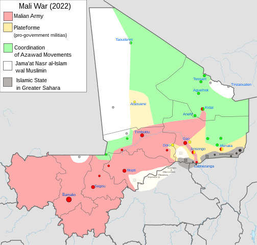 |
|---|
| A map of the Mali war. Image obtained here. |
In conclusion, we used SQL queries to investigate various demographic trends among countries. We studied some outliers in the dataset, computed population density and expected population growth, and finally, we took a closer look at countries with high death rates.
We found that many ongoing conflicts have a noticable impact in terms of number of deaths per 1,000 people. For countries whose conflicts have occured more recently, such as the Russia-Ukraine conflict, the number of new births per 1,000 people remains relatively small, when compared to other countries with high death rates. For other countries with high death rates, their low population density combined with high birth rate suggests an impoverished, rural setting where children are needed for labor purposes, and armed conflicts often persist.
To learn more about ongoing conflicts and causes for high death rates within a few countries discussed in this notebook, please visit the following links: Mali War, Somali Civil War, Russian Invasion of Ukraine, Addressing Causes of Mortality in Zambia. Thank you for reading this notebook!